Countercyclical capital buffer (CCyB)

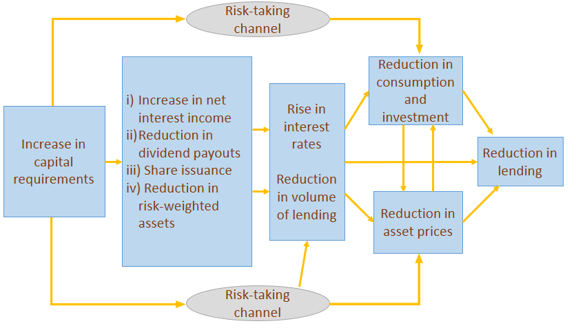
This capital buffer is a macroprudential requirement additional to microprudential capital requirements and other macroprudential buffers. It is designed to curb the growth of cyclical systemic risk and bolster banks’ solvency so that they can absorb any losses should systemic risks arise.

The activation of this capital requirement ensures that banks take actions (e.g. lowering the volume of lending and raising rates, taking on less risk) that moderate the credit cycle. This also results in a lower intensity of the real business cycle (consumption and investment) and a downward correction to financial asset prices, which in turn further moderates the credit cycle.

Note: See A. Estrada and J. Mencía (2021), “El cuadro de mandos de la Política Macroprudencial  (377 KB)", Información Comercial Española, No 918, 2021. (Only available in Spanish).

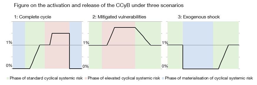
Following the 2024 revision  (392 KB) of the methodological framework for setting the CCyB, this buffer will be set at 1% when cyclical systemic risks are at a standard level (an intermediate level between high and low risk). The buffer will be increased to levels above 1% when cyclical systemic risk is high (above the standard level) (see panels 1 and 2 of the figure).

When these high systemic risks are mitigated and return to a standard level, the CCyB will be gradually released until it reaches 1% (see panel 2 of the figure).

The CCyB would also be released, generally in full, following the materialisation of cyclical (panel 1) or other (panel 3) systemic risks. This release would help to mitigate the adverse impact of crises on the provision of credit to the real economy and to contain the possible materialisation of additional cyclical systemic risks in such stressed settings.

After a crisis (see panels 1 and 3 of the figure), the build-up from 0% to 1% must take place gradually over several periods, and only if cyclical systemic risk indicators return to a standard level.

The CCyB can be activated for credit exposures as a whole or for certain sectors where imbalances have been identified.

Activation of the CCyB during standard cyclical risk phases incurs very limited costs in terms of loss of credit and GDP growth. Conversely, the release of the CCyB during periods of macro-financial crisis results in substantial benefits in the form of less severe contractions in these variables.

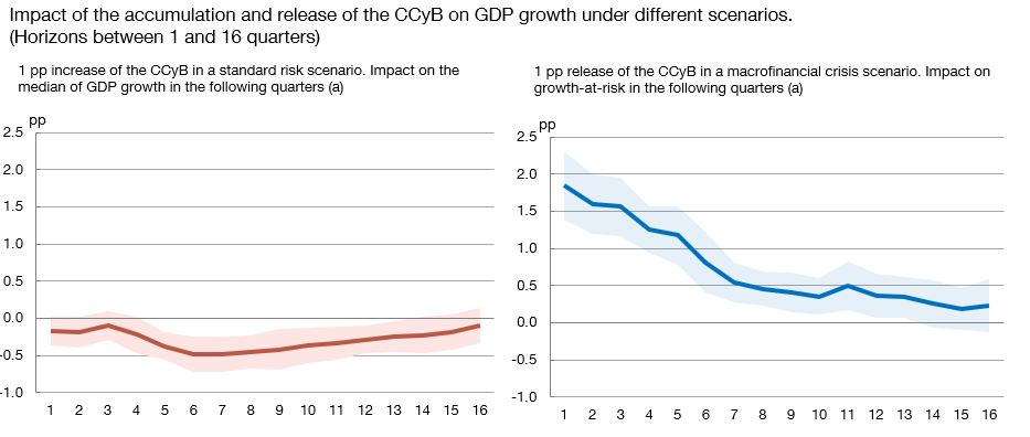
SOURCE: Banco de España.
a. The lines represent the percentage point impact of a 1 pp increase (left-hand panel) and decrease (right-hand panel) in the combined buffer requirement (CBR) on the 50th (left-hand panel) and 10th (right-hand panel) percentiles of the annualised GDP growth distribution, between the time of the change in the CBR and different horizons (from 1 to 16 quarters). The shaded areas represent the 95% confidence intervals for the estimates. The horizontal axis shows the quarters elapsed since the change in the CBR. GDP growth and financial risk are assumed to be consistent with a standard risk scenario in the left-hand panel and a macro-financial crisis scenario in the right-hand panel, drawing on their historical distributions in Spain between 1990 and 2019. For more details, see Ángel Estrada et al. (2024). “Analysis of cyclical systemic risks in Spain and of their mitigation through countercyclical bank capital requirements”. Documentos Ocasionales, 2414, Banco de España.

Decisions on these instruments are made in two stages, following a guided discretion approach:

1. Analysis of a scoreboard of 16 key indicators  (28 KB), grouped into four blocks (macroeconomic, macro-financial, market and banking system). These indicators are analysed individually (as in the case of the credit-to-GDP and output gaps), as well as on an aggregated basis using composite indicators.
2. Analysis of additional quantitative and qualitative information available, to confirm or rectify the outcome of the first stage.

Composite indicators by risk category

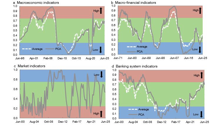
SOURCE: Datastream, INE, Banco de España and own calculations.
Note: The key indicators for monitoring cyclical risk are aggregated for each of the main risk categories. The white lines depict an aggregation through simple averages and the grey lines an aggregation based on principal component analysis (PCA). Both aggregation methodologies are described in Ángel Estrada et al. (2024). “Analysis of cyclical systemic risks in Spain and of their mitigation through countercyclical bank capital requirements”. Documentos Ocasionales, 2414, Banco de España. The IRS indicator aggregates 12 financial market variables based on the methodology described in Box 1.1 of the May 2013 Financial Stability Report. Each indicator is defined, on a scale between 0 and 1, based on its percentile relative to its historical distribution. The blue (green) [red] range corresponds to a low (standard) [high] cyclical systemic risk level or, in the case of banking system indicators, capital generation capacity by the banking system.

Overall composite indicator

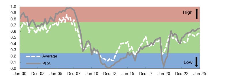
SOURCE: Datastream, INE, Banco de España and own calculations.
Note: Key indicators for monitoring cyclical systemic risk are aggregated in a single composite indicator. The white line depicts an aggregation through simple averages and the grey line an aggregation based on principal component analysis (PCA). Both aggregation methodologies are described in Ángel Estrada et al. (2024). “Analysis of cyclical systemic risks in Spain and of their mitigation through countercyclical bank capital requirements”. Documentos Ocasionales, 2414, Banco de España. Each indicator is defined, on a scale between 0 and 1, based on its percentile relative to its historical distribution. The blue (green) [red] range corresponds to a low (standard) [high] cyclical systemic risk level.

Selected key indicators for monitoring CCyB decisions

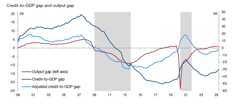
SOURCE: INE, Banco de España and own calculations.
Note: The areas shaded in grey show the two crisis periods identified in Spain since 2009: a systemic banking crisis (the most recent one, from 2009 Q1 to 2013 Q4) and the economic crisis triggered by the outbreak of the COVID-19 pandemic (from 2020 Q1 to 2021 Q4). The output gap is the percentage difference between the actual and potential level of GDP. Values calculated in constant 2010 prices. See Pilar Cuadrado and Enrique Moral-Benito. (2016). “Potential growth of the Spanish economy  (443 KB)”. Documentos Ocasionales, 1603, Banco de España. The credit-to-GDP gap is calculated as the percentage point difference between the observed ratio and its long-term trend calculated by applying a one-sided Hodrick-Prescott statistical filter with a smoothing parameter equal to 25,000. This parameter is calibrated to match the financial cycles historically observed in Spain. See Jorge E. Galán. (2019). “Measuring credit-to-GDP gaps. The Hodrick-Prescott revisited  (1 MB)”.  Documentos Ocasionales, 1906, Banco de España.

• Data download  (6 KB)

Other complementary indicators include, for example, credit intensity, price gaps in the real estate sector and other measures of house price imbalances, the non-financial private sector’s debt service and ROE both at consolidated level and for business in Spain.

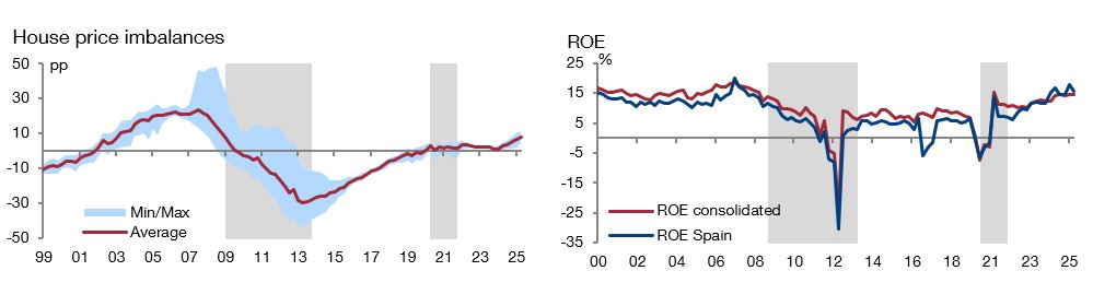
SOURCE: INE, Banco de España and own calculations.
Note: The areas shaded in grey show the two crisis periods identified in Spain since 2009: a systemic banking crisis (the most recent one, from 2009 Q1 to 2013 Q4) and the economic crisis triggered by the outbreak of the COVID-19 pandemic (from 2020 Q1 to 2021 Q4). The house price imbalance ranges shown are the lowest and highest values of a set of indicators of residential real estate sector price developments relative to their long-term trends (some of these indicators have been obtained using a statistical filter and others using econometric models).

• Data download  (9 KB)